09.4g: Dataflow

Dataflow is a managed runner that supports Apache Beam workloads. Beam is an open-source project spun out of Google to implement large scale processing of both stream and batch workloads. Beam uses a transform-based processing approach and has a programming paradigm that is similar to a functional programming one where functions do not maintain state. Beam computations are expressed in graph-like form. Input flows into the graph, is transformed via computations within nodes of the graph, and then output via nodes that serve as sinks for the results. The abstraction is useful for applications such as log ingestion and analysis from a web site or sensor data ingestion from IoT devices. One of the features of Dataflow is its ability to be 'serverless'. Processing capacity is dynamically brought up and down as the computation within the graph proceeds. This is in contrast to our prior Dataproc labs in which clusters must be explicitly allocated and deallocated by the operator.

In this lab, we'll demonstrate the programming model in action using a simple program that determines the top packages included in a Java code base.

First, clone the repository containing the code and change into its directory:

git clone https://github.com/GoogleCloudPlatform/training-data-analyst.git

cd training-data-analyst/courses/machine_learning/deepdive/04_features/dataflow/python/

Then, create a Python virtual environment and activate it.

python3 -m venv env
source env/bin/activate

Install the Apache Beam package that is configured for execution on Google Cloud Platform. In addition, since we will eventually deploy our pipelines onto GCP, an OAuth client package must be installed so our program can use the credentials we supply it to authorize its access on our project.

pip install -U pip
pip install apache-beam[gcp] oauth2client==3.0.0

Dataflow transforms can be mapped onto their own compute nodes for execution. In Python, this is done with special syntax. Consider the code below for a pipeline that performs a string search (e.g. grep). The code instantiates p, a Beam pipeline, and configures variables specifying its input sources, output sinks, and a search term. It then specifies an expression for the computation that takes file names from input and reads lines from them (beam.io.ReadFromText(input)), checks to see if the lines start with the searchTerm (beam.FlatMap(lambda line: my_grep(line, searchTerm)), then writes the lines out to a directory (beam.io.WriteToText(output_prefix)). The expression is then evaluated via p.run().

grep.py

import apache_beam as beam
import sys

def my_grep(line, term):
   if line.startswith(term):
      yield line

p = beam.Pipeline(argv=sys.argv)
input = '../*.java'
output_prefix = '/tmp/...'
searchTerm = 'import'

(p
   | 'GetJava' >> beam.io.ReadFromText(input)
   | 'Grep' >> beam.FlatMap(lambda line: my_grep(line, searchTerm) )
   | 'write' >> beam.io.WriteToText(output_prefix)
)

p.run().wait_until_finish()

Bring up is_popular.py in the code editor.

edit is_popular.py

Reverse-engineer the code and make note of where the input is taken from and where the output goes to by default.

Answer the following questions for your lab notebook.

Where is the input taken from by default?
Where does the output go by default?
Examine both the getPackages() function and the splitPackageName() function. What operation does the 'PackageUse()' transform implement?
Look up Beam's CombinePerKey. What operation does the TotalUse operation implement?

The operations in the pipeline mimic a Map-Reduce pattern, demonstrating Beam's ability to support it.

Answer the following questions for your lab notebook.

Which operations correspond to a "Map"?
Which operation corresponds to a "Shuffle-Reduce"?
Which operation corresponds to a "Reduce"?

Go back to Cloud Shell and run the pipeline.

python is_popular.py

Go to where the output file is written out and cat the file.

Take a screenshot of its contents
Explain what the data in this output file corresponds to based on your understanding of the program.

In this lab, we'll be running a word counting example directly from the Apache Beam package. The code can be run locally as well as executed on nodes in GCP's Dataflow service, a managed runner that supports Apache Beam pipelines. We'll be running a word counting example from the Apache Beam package. Ensure you have activated the Python environment used in the previous lab.

When using Python virtual environments, packages are installed within the environment's directory. In the directory that you have created the Python virtual environment, bring up the code for the wordcount example that comes with the Python package.

edit env/lib/python3.*/site-packages/apache_beam/examples/wordcount.py

When the code is invoked as a module, it executes the run() function. Within the function, a pipeline p is incrementally constructed using the Beam syntax (lines, counts, output) before the entire pipeline is executed via p.run(). Examine the code that implements the function and answer the following questions for your lab notebook:

What are the names of the stages in the pipeline?
Describe what each stage does.

We'll first run the pipeline locally in Cloud Shell. In this case, we use the -m flag to have Python execute the module directly, specifying the output prefix as outputs.

python -m apache_beam.examples.wordcount \
  --output outputs

After running the script, perform the following and show a screenshot of the results in your lab notebook:

Use wc with an appropriate flag to determine the number of different words in King Lear.
Use sort with appropriate flags to perform a numeric sort on the key field containing the count for each word in descending order. Pipe the output into head to show the top 3 words in King Lear and the number of times they appear

The pipeline specified treats every word as is. As a result, it is case-sensitive, leading to 'King' and 'KING' having distinct counts. Go back to the code editor and edit wordcount.py. Find a place in the pipeline that you can insert a stage that transforms all of the characters it receives into lowercase. The snippet below can be used:

      | 'lowercase' >> beam.Map(lambda x: x.lower())

Perform the following and show a screenshot of the results in your lab notebook:

Use the previous method to show the top 3 words in King Lear, case-insensitive, and the number of times they appear.

Cloud Dataflow can be used to execute the pipeline in parallel in an on-demand, "serverless" fashion. To use Dataflow, we must enable the APIs for the lab. Dataflow requires Compute Engine instances to execute the code and storage buckets to store the results so those components must also be enabled.

gcloud services enable dataflow compute_component storage_component storage_api

Throughout the codelab, we'll be referencing our storage bucket and our desired region in environment variables. The commands below will do so by configuring our bucket to be the name of our project and the region to be us-west1.

export BUCKET=${GOOGLE_CLOUD_PROJECT}
export REGION=us-west1

Then, create the storage bucket if it hasn't been created already.

gsutil mb gs://${BUCKET}

We will need to create a service account to run our workload with. Change into your home directory and use gcloud to create a service account named df-lab.

cd

gcloud iam service-accounts create df-lab

To run a Dataflow pipeline, we require permissions across several IAM roles. Specifically, we add:

roles/dataflow.admin to create and manage Dataflow jobs
roles/dataflow.worker to create Compute Engine VMs (workers) on-demand to run the Dataflow pipeline.
roles/storage.admin to create storage buckets for the results
roles/iam.serviceAccountUser to create Compute Engine VMs that use a specific service account
roles/serviceusage.serviceUsageConsumer to use platform services.

gcloud projects add-iam-policy-binding ${GOOGLE_CLOUD_PROJECT} \
  --member serviceAccount:df-lab@${GOOGLE_CLOUD_PROJECT}.iam.gserviceaccount.com \
  --role roles/dataflow.admin

gcloud projects add-iam-policy-binding ${GOOGLE_CLOUD_PROJECT} \
  --member serviceAccount:df-lab@${GOOGLE_CLOUD_PROJECT}.iam.gserviceaccount.com \
  --role roles/dataflow.worker

gcloud projects add-iam-policy-binding ${GOOGLE_CLOUD_PROJECT} \
  --member serviceAccount:df-lab@${GOOGLE_CLOUD_PROJECT}.iam.gserviceaccount.com \
  --role roles/storage.admin

gcloud projects add-iam-policy-binding ${GOOGLE_CLOUD_PROJECT} \
  --member serviceAccount:df-lab@${GOOGLE_CLOUD_PROJECT}.iam.gserviceaccount.com \
  --role roles/iam.serviceAccountUser

gcloud projects add-iam-policy-binding ${GOOGLE_CLOUD_PROJECT} \
 --member serviceAccount:df-lab@${GOOGLE_CLOUD_PROJECT}.iam.gserviceaccount.com \
 --role roles/serviceusage.serviceUsageConsumer

Once the service account has the necessary policies attached, we will create a service account key (df-lab.json) that will allow us to access the df-lab account.

gcloud iam service-accounts keys create df-lab.json --iam-account df-lab@${GOOGLE_CLOUD_PROJECT}.iam.gserviceaccount.com

We must also set the environment variable that can be used by our Python environment to access the service account key.

export GOOGLE_APPLICATION_CREDENTIALS=$PWD/df-lab.json

We can now repeat our execution, but rather than use a local runner, we can specify a DataflowRunner and a set of locations for the pipeline to take input from and to store results to.

python -m apache_beam.examples.wordcount \
  --region ${REGION} \
  --input gs://dataflow-samples/shakespeare/kinglear.txt \
  --output gs://$BUCKET/results/outputs \
  --runner DataflowRunner \
  --project ${GOOGLE_CLOUD_PROJECT} \
  --temp_location gs://${BUCKET}/tmp/

After executing the program, which takes around 5 minutes to complete, visit Dataflow in the web console and click on the Dataflow job that was executed. Examine both "Job Graph" and "Job Metrics".

Include the following in your lab notebook:

The part of the job graph that has taken the longest time to complete.
The autoscaling graph showing when the worker was created and stopped.
Examine the output directory in Cloud Storage. How many files has the final write stage in the pipeline created?

Delete the IAM policies and the service account.

gcloud projects remove-iam-policy-binding ${GOOGLE_CLOUD_PROJECT} \
  --member serviceAccount:df-lab@${GOOGLE_CLOUD_PROJECT}.iam.gserviceaccount.com \
  --role roles/dataflow.admin

gcloud projects remove-iam-policy-binding ${GOOGLE_CLOUD_PROJECT} \
  --member serviceAccount:df-lab@${GOOGLE_CLOUD_PROJECT}.iam.gserviceaccount.com \
  --role roles/dataflow.worker

gcloud projects remove-iam-policy-binding ${GOOGLE_CLOUD_PROJECT} \
  --member serviceAccount:df-lab@${GOOGLE_CLOUD_PROJECT}.iam.gserviceaccount.com \
  --role roles/storage.admin

gcloud projects remove-iam-policy-binding ${GOOGLE_CLOUD_PROJECT} \
  --member serviceAccount:df-lab@${GOOGLE_CLOUD_PROJECT}.iam.gserviceaccount.com \
  --role roles/iam.serviceAccountUser

gcloud projects remove-iam-policy-binding ${GOOGLE_CLOUD_PROJECT} \
  --member serviceAccount:df-lab@${GOOGLE_CLOUD_PROJECT}.iam.gserviceaccount.com \
  --role roles/serviceusage.serviceUsageConsumer

gcloud iam service-accounts delete df-lab@${GOOGLE_CLOUD_PROJECT}.iam.gserviceaccount.com

Delete the storage bucket

gsutil -m rm -r gs://${BUCKET}

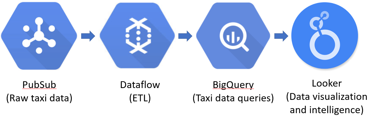
Dataflow is often used within an ETL (Extract-Transform-Load) pipeline to ingest raw streaming data into a backend data warehouse. In this lab, we'll be showing a simple example of this pattern that is commonly employed in Data Science workflows to take raw data that is being collected and to turn it into actionable business intelligence (BI).

In this lab, you will subscribe to a raw, real-time data stream of taxi rides being taken in New York City. The data stream is part of Google Cloud's public dataset and ride data is continuously being published onto a publicly accessible Google Cloud PubSub topic. From this stream, you'll deploy a continuously running ETL pipeline in Dataflow that extracts the data in the stream and transforms it into clean records to be inserted into the BigQuery data warehouse. Finally, you will run simple queries on the data and then visualize it using the Looker data studio.

In Cloud Shell, if you have not yet enabled PubSub on the project, enable it.

gcloud services enable pubsub

Then, create a subscription that subscribes to the raw taxi data located on the public PubSub topic projects/pubsub-public-data/topics/taxirides-realtime

gcloud pubsub subscriptions create taxisub \
  --topic=projects/pubsub-public-data/topics/taxirides-realtime

Then, pull and acknowledge the receipt of one message from the raw data stream. Examine the data returned.

gcloud pubsub subscriptions pull taxisub --auto-ack

The data that is returned is a JSON object.

Take a screenshot listing the different fields of this object.

The goal of our ETL pipeline will be to extract these fields and load them into a backend table in our data warehouse.

Delete the subscription.

gcloud pubsub subscriptions delete taxisub

We'll first set up the BigQuery dataset and table that will ingest the taxi data from the raw stream. Within Cloud Shell, create a dataset named taxirides.

bq mk taxirides

Then, create a table within the dataset named realtime to load the taxi ride data into. Note that we specify the schema for this table that aligns with the results of the ETL pipeline. In this case, the pipeline simply maps fields of the JSON into columns in our table as shown in the schema we include.

bq mk \
  --time_partitioning_field timestamp \
  --schema ride_id:string,point_idx:integer,latitude:float,longitude:float,\
timestamp:timestamp,meter_reading:float,meter_increment:float,ride_status:string,\
passenger_count:integer \
  -t taxirides.realtime

Finally, create a storage bucket for use by the Dataflow service to stage intermediate data.

gsutil mb gs://${GOOGLE_CLOUD_PROJECT}-taxi

Dataflow comes with a number of pipeline templates that represent common tasks one would implement. One such template ingests data from a PubSub topic into BigQuery, as we are attempting to do with the taxiride data. The template is located at gs://dataflow-templates/latest/PubSub_to_BigQuery. Templates such as this one are akin to a "Zero-ETL" approach for data management since the extraction and loading of data is done automatically by the platform itself.

Bring up a serverless Dataflow pipeline using this template that will continuously read taxi ride data sent to the PubSub topic and load it into the BigQuery table created in the previous step using the template.

gcloud dataflow jobs run taxirides \
    --gcs-location gs://dataflow-templates/latest/PubSub_to_BigQuery \
    --region us-west1 \
    --staging-location gs://${GOOGLE_CLOUD_PROJECT}-taxi/tmp \
    --parameters inputTopic=projects/pubsub-public-data/topics/taxirides-realtime,\
outputTableSpec=${GOOGLE_CLOUD_PROJECT}:taxirides.realtime

Then, visit the Cloud Dataflow console in the web UI and view the running job. Wait until the job is functioning and has processed 5-10 minutes worth of raw data from the stream..

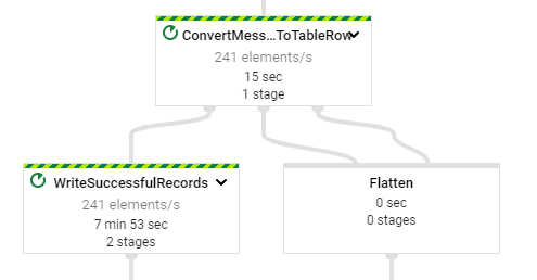
Take a screenshot of the pipeline that includes its stages and the number of elements per second being handled by individual stages.

Stop the Dataflow job when a sufficient amount of data has been collected. One can use the web console or Cloud Shell to do so. For Cloud Shell, find the job's ID via the command below.

gcloud dataflow jobs list --status=active

Then, making note of the JOB_ID, cancel the job.

gcloud dataflow jobs cancel <JOB_ID> --region=us-west1

Visit the BigQuery web console and navigate to the table we've created within our project at taxirides:realtime. Examine the table.

Take a screenshot showing the number of passengers and the amount paid for the first ride
Take a screenshot showing the estimated number of rows in the table.

The table contains raw ride data, but in many cases, it is difficult to provide any meaningful insight on it without further processing. One of the functions that business intelligence tools provide is the ability to perform data querying and visualization on the raw data. We'll be emulating this using BigQuery and the Looker Studio data visualization tool.

First, query the table to obtain the number of rides, number of passengers, and amount of revenue for rides that have been taken during the collection period in BigQuery.

SELECT
  FORMAT_TIMESTAMP("%R", timestamp, "America/Los_Angeles") AS minute,
  COUNT(DISTINCT ride_id) AS total_rides,
  SUM(passenger_count) AS total_passengers,
  SUM(meter_reading) AS total_revenue
FROM
  taxirides.realtime
WHERE
  ride_status = 'dropoff'
GROUP BY
  minute
ORDER BY
  minute ASC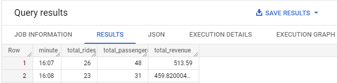

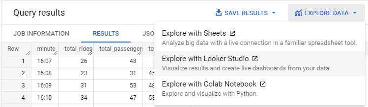
Take a screenshot showing the per-minute number of rides, passengers, and revenue for the data collected

There are several options for examining the data from the query we've run. One tool for doing so that has been integrated into Google Cloud Platform is Looker Studio: a tool for generating interactive dashboards for easily generating reports and visualizations on data. From the query results of the prior query, click on "Explore Data" and bring up the query results in Looker Studio.

Then, create a Column Chart that plots the time in minutes over ascending time on the x-axis and the total number of rides and revenue on the y-axis by configuring the Dimension, Metrics, and Sort criteria of the chart similar to that shown below.

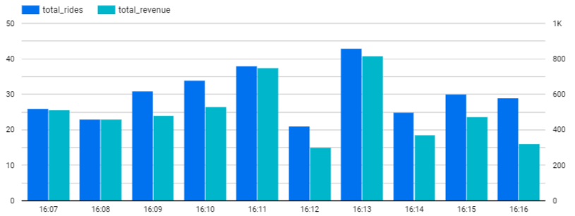
Take a screenshot showing the plot for your data for your lab notebook

Delete the BigQuery table and dataset

bq rm taxirides.realtime
bq rm taxirides

Delete the staging storage bucket

gsutil rm -r gs://${GOOGLE_CLOUD_PROJECT}-taxi